Understand and Implement an Artificial Neural Network from Scratch

TL;DR Understand and implement an artificial neural network from scratch using NumPy, learn the basics of feedforward and backpropagation, and explore the impact of changing parameters during training.

Generated with Bing DALL-E 3

Artificial intelligence is a hype topic. But what is behind the powerful networks of the big tech companies? An artificial neural network (ANN) is usually implemented with frameworks such as TensorFlow, Keras or PyTorch. Such frameworks are suitable for very complex ANNs. As a data scientist, however, it is essential to understand the basics.

This article aims to help you understand how a neural network works. First, we introduce the basics of an ANN in general. Then we look at the basic concepts of ANNs in detail. After that, we explain how to implement a neural network with NumPy using binary classification. We will also do some experiments to help you understand how neural networks work.

After reading this article, you should have a basic understanding of how artificial neural networks work.

Artificial Neural Networks in general

An artificial neural network uses biology as a model. Such a network consists of artificial neurons (also called nodes) and connections (also called edges) between these neurons. A neural network has one or more hidden layers, each layer consisting of several neurons.

Each neuron in each layer receives the output of each neuron in the previous layer as input. Each input to the neuron is weighted. The following figure shows a Feed Forward Neural Network. In such a network, the connections between the nodes are acyclic.

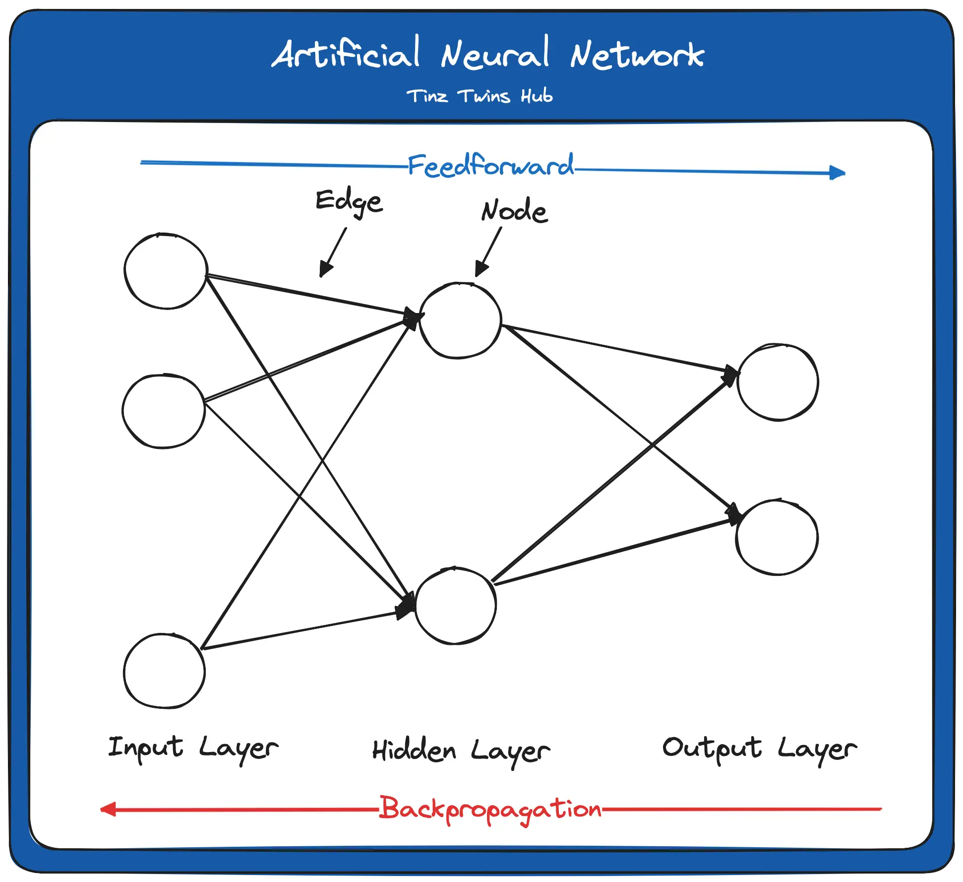
The important terms are marked in bold italics and will be looked at in more detail in this article. Feedforward is the flow of the input data through the neural network from the input layer to the output layer. As it passes through the individual layers of the network, the input data is weighted at the edges and normalized by an activation function. The weighting and the activation function are part of a neuron.

The calculated values at the output of the network have an error compared to the true result values. In our training data, we know the true result values. The return of the errors is called backpropagation, where the errors are calculated per node. The gradient descent method is usually used to minimize the error terms. The training of the network with backpropagation is repeated until the network has the smallest possible error.

Then the trained neural network can be used for a prediction on new data (test data). The quality of the prediction depends on many factors. As a data scientist, you need to pay attention to data quality when training a network.

---

---

Concept of a Perceptron

The concept of a perceptron was first introduced by Frank Rosenblatt in 1957. A perceptron consists of an artificial neuron with adjustable weights and a threshold. For a better understanding, we explain how a perceptron works with the following figure.

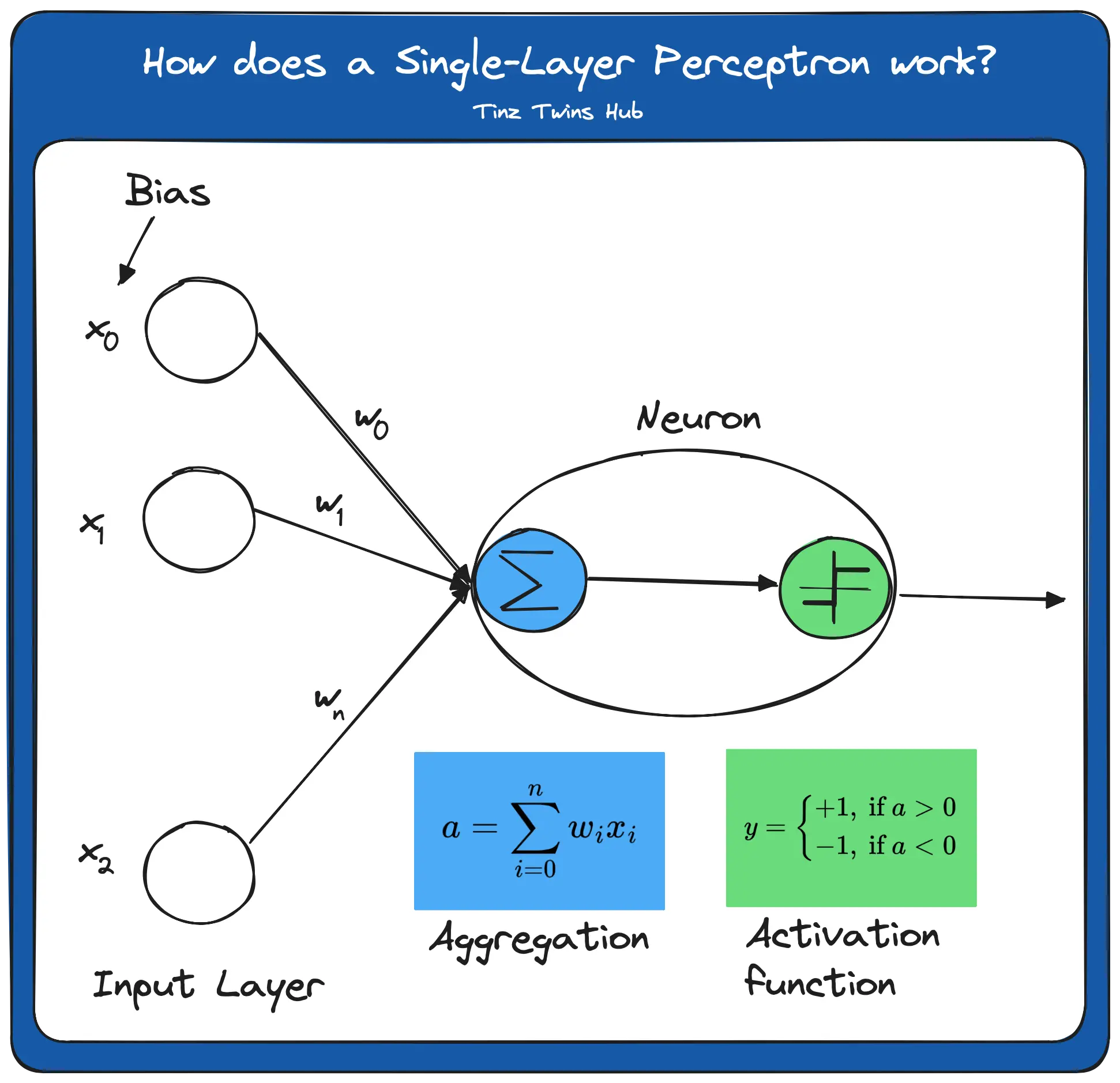
The figure illustrates an input layer and an artificial neuron. The input layer contains the input value and x_0 as bias. In a neural network, a bias is required to shift the activation function either to the positive or negative side. The perceptron has weights on the edges. The weighted sum of input values and weights is then calculated. It is also known as aggregation. The result a finally serves as input into the activation function.

In this simple example, the step function is used as the activation function. Here, all values of a > 0 map to 1 and values a < 0 map to -1. There are different activation functions. Without an activation function, the output signal would just be a simple linear function. A linear equation is easy to solve, but it is very limited in complexity and has much less ability to learn a complex function mapping from data. The performance of such a network is severely limited and gives poor results.

Feedforward

Feedforward is the flow of input data through the neural network from the input layer to the output layer. This procedure is explained in the following figure:

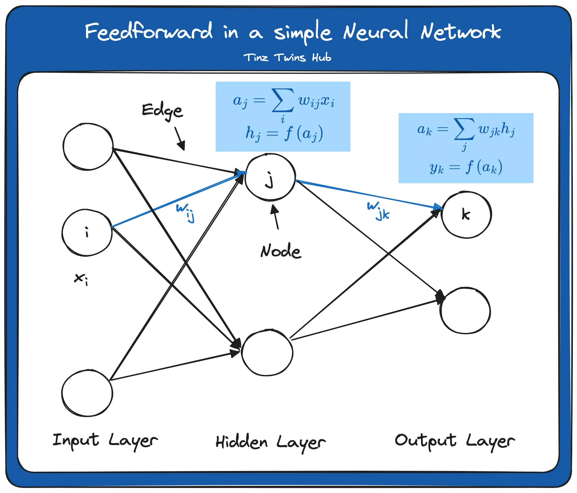
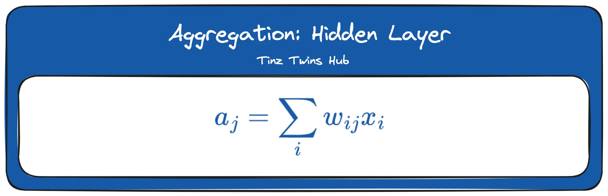
In this example, we have exactly one hidden layer. First, the data x enters into the input layer. x is a vector with individual data points. The individual data points are weighted with the weights of the edges. There are different procedures for initializing the starting weights, which we will not discuss in this article. This step is called aggregation. Mathematically, this step is as follows:

The result of this step serves as the input of the activation function. The formula is:

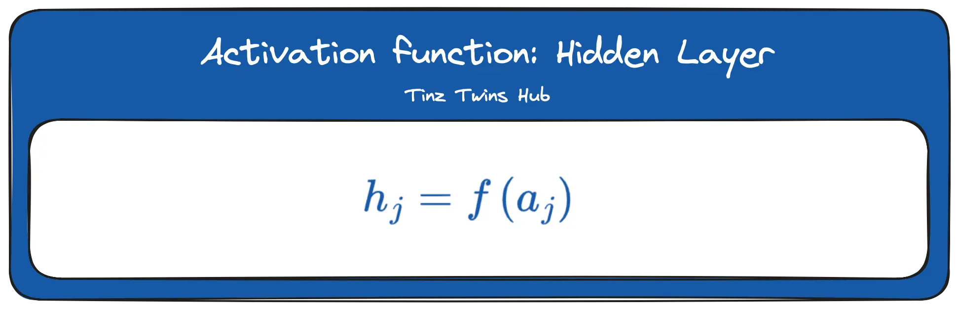
We denote the activation function by f. The result from the activation function finally serves as input for the neuron in the output layer.

This neuron again performs an aggregation. The formula is as follows:

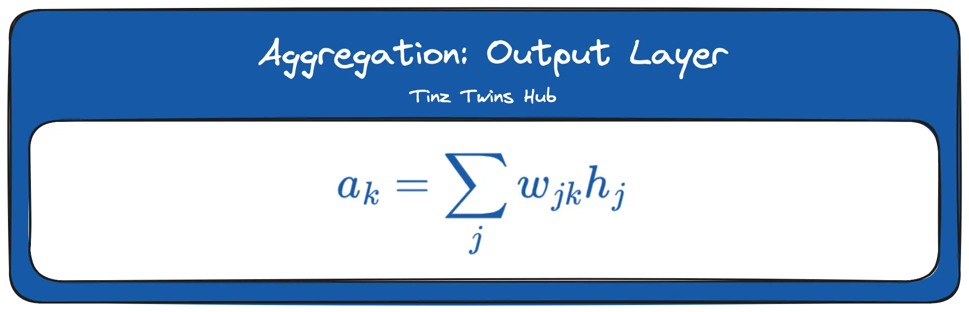
The result is again the input for the activation function. The formula is:

We denote the output of the network by y. y is a vector with all y_k. The activation function in the hidden layer and the output layer does not have to be identical. In practice, different activation functions are suitable depending on the use case.

---

---

Gradient descent method

The gradient descent method minimizes the error terms. In this context, the error function is derived to find a minimum. The error function calculates the error between calculated and true result values.

First, the direction in which the curve of the error function slopes most sharply must be determined. That is the negative gradient. A gradient is a multidimensional derivative of a function. Then we walk a bit in the direction of the negative slope and update the weights. The following formula illustrates this procedure:

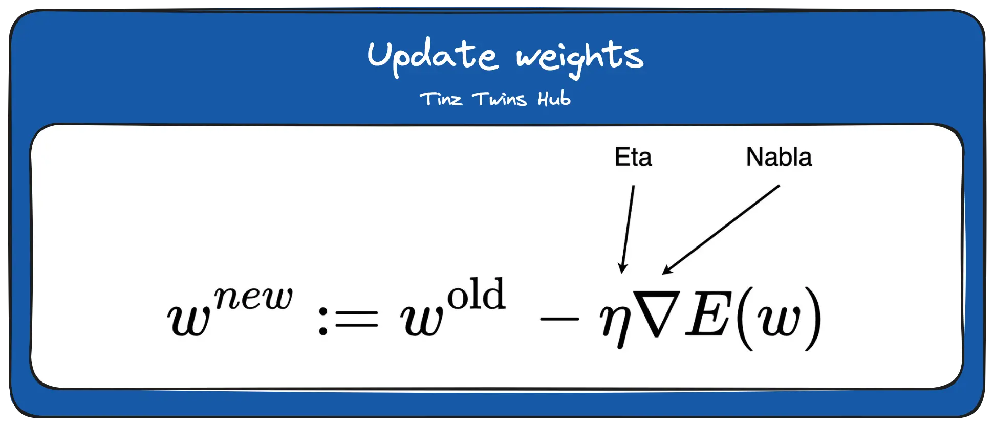
The inverted triangle is the Nabla sign and is used to indicate derivatives of vectors. The gradient descent method still requires a learning rate (Eta sign) as a transfer parameter. The learning rate specifies how strongly the weights are adjusted. E is the error function that is derived. This whole process repeats until there is no more significant improvement.

Backpropagation

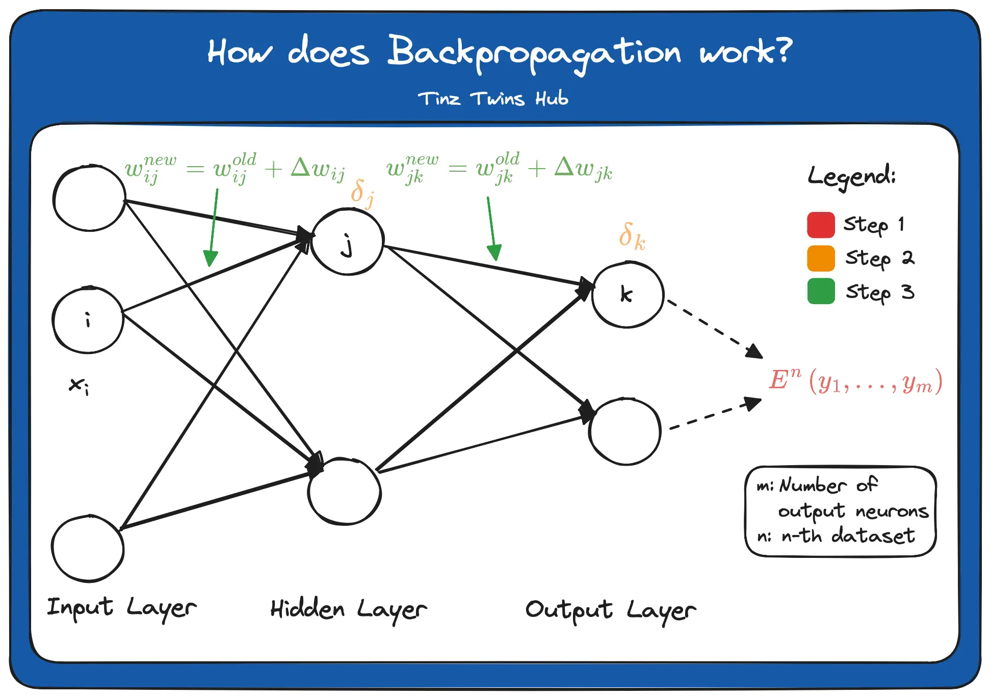
In principle, Backpropagation can be divided into three steps.

1. Step: Construct the error function
2. Step: Calculate the error term for each node on the output and hidden layer
3. Step: Update the weights on the edges

Construct the error function

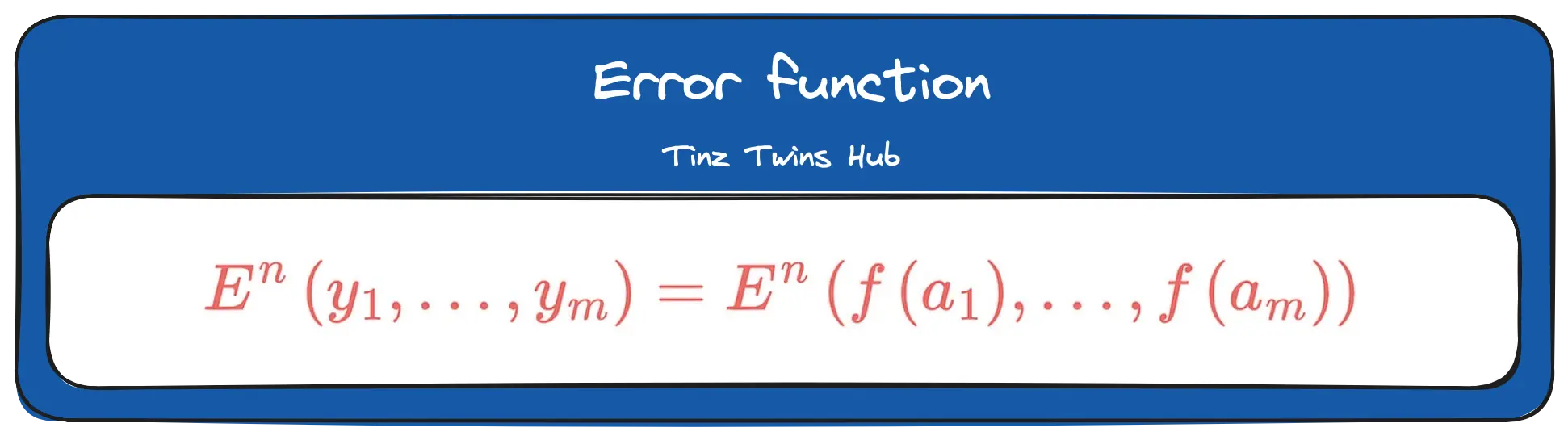
The calculated values at the output of the network have an error compared to the true result values. An error function is used to calculate this error. Mathematically, the error can be calculated in different ways. The error function contains the result from the output layer as input. That means that the whole calculation of the feedforward is used as an input to the error function. The n of the function E denotes the n-th data set. m represents the number of output neurons.

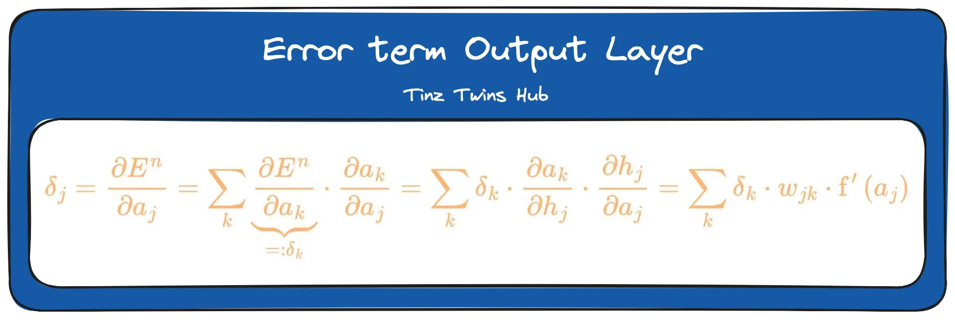
Calculate the error term for each node on the output and hidden layer

The error terms are marked orange in the Backpropagation figure. To calculate the error terms for the output layer, we have to derive the error function according to the respective weights. For this, we use the chain rule. Mathematically, it looks like this:

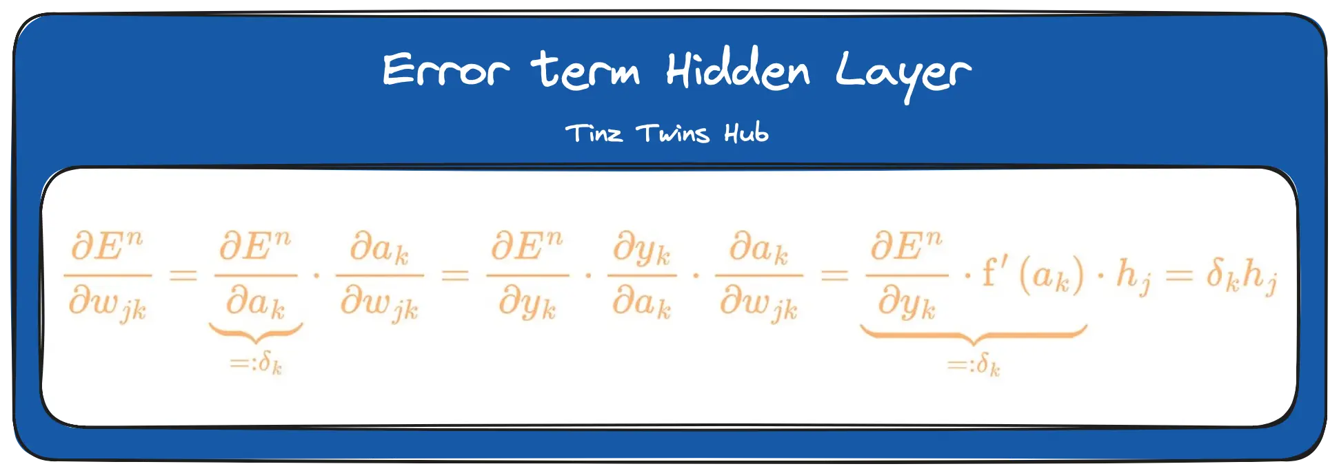
To calculate the error terms for the hidden layer, we derive the error function according to a_j.

Update of the weights on the edges

The new weights between the hidden and output layers can now be calculated using the respective error terms and a learning rate. Through the minus (-), we go a bit into the direction of the descent.

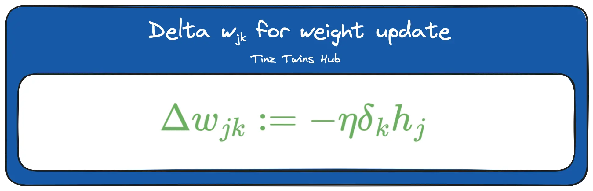
The triangle is the Greek letter delta. In mathematics and computer science, this letter is used to indicate the difference. Furthermore, we can now update the weights between the input and hidden layer. The formula looks like this:

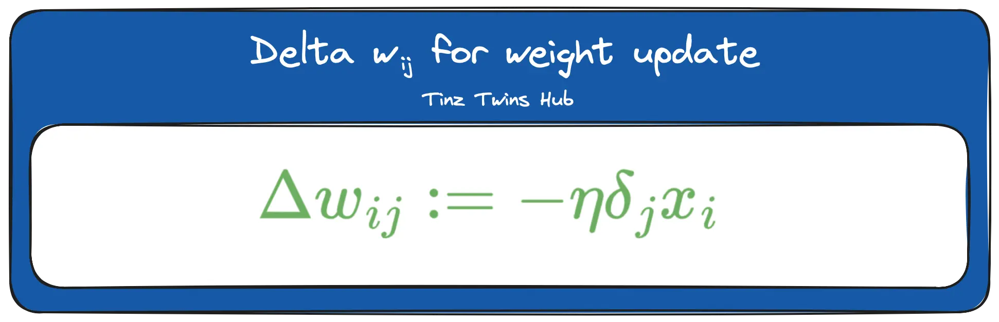
The deltas are used for the weight updates, as shown in the figure at the beginning of the Backpropagation section.

---

---

Implement an artificial neural network with NumPy

1. Step — Technical requirements

You will need the following prerequisites:

• Access to a bash (macOS, Linux or Windows).
• Installed Python (≥ 3.7)
• A Python package manager of your choice like conda
• Code editor of your choice (We use VSCode.)

Setup

• Create a conda environment (env): conda create -n neural-network python=3.9.12 -> Answer the question Proceed ([y]/n)? with y.
• Activate the conda env: conda activate neural-network
• Install the necessary libraries: pip install matplotlib==3.7.1 numpy==1.24.2 plotly==5.14.1 pandas==2.0.0 scikit-learn==1.2.2

2. Step — Imports

In the second step, we import all requirements. For the visualizations, we use matplotlib and Plotly. In the last line, we set the figure size of the matplotlib plots.

import numpy as np
import sklearn
import sklearn.datasets
from sklearn.model_selection import train_test_split
from sklearn.metrics import roc_curve, auc
from sklearn.metrics import accuracy_score
import pandas as pd
import plotly.express as px
import time
import matplotlib.pyplot as plt
%matplotlib inline
import matplotlib
matplotlib.rcParams['figure.figsize'] = (5.0, 4.0)

3. Step — Generate the dataset

We use the simple toy dataset sklearn.datasets.make_moons. You can find more information about the dataset on the sklearn website.

The function has the following parameters:

• n_samples: Total number of generated points
• noise: Standard deviation of Gaussian noise added to the data
• random_state: Seed for reproducible output

n = 1000
data_seed = 4242   # choose seed value

X, y = sklearn.datasets.make_moons(
    n_samples = n, 
    noise = 0., 
    random_state = data_seed)

plt.scatter(
    x = X[:,0], 
    y = X[:,1], 
    s = 40,   # marker size
    c = y)

Scatter-Plot:

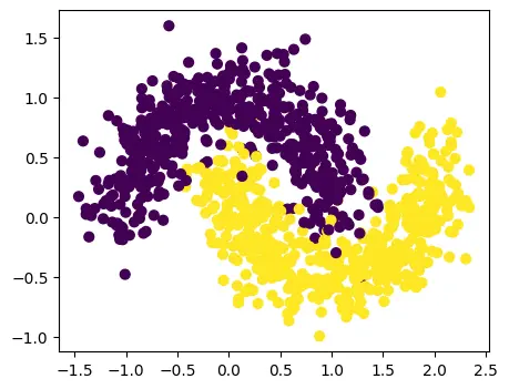
We see two interleaving half circles.

4. Step — Split the dataset

In this step, we use the train_test_split()function of the sklearn package to create our training and test dataset with labels.

The function has the following parameters:

• X: The moons dataset
• y: The labels
• test_size: Size of the test dataset in percent
• random_size: Seed for reproducible output

test_size = 0.25
split_seed = 42 # choose split seed value

X_train, X_test, y_train, y_test = train_test_split(
    X,
    y,
    test_size = test_size,
    random_state = split_seed)

5. Step — Define helper functions

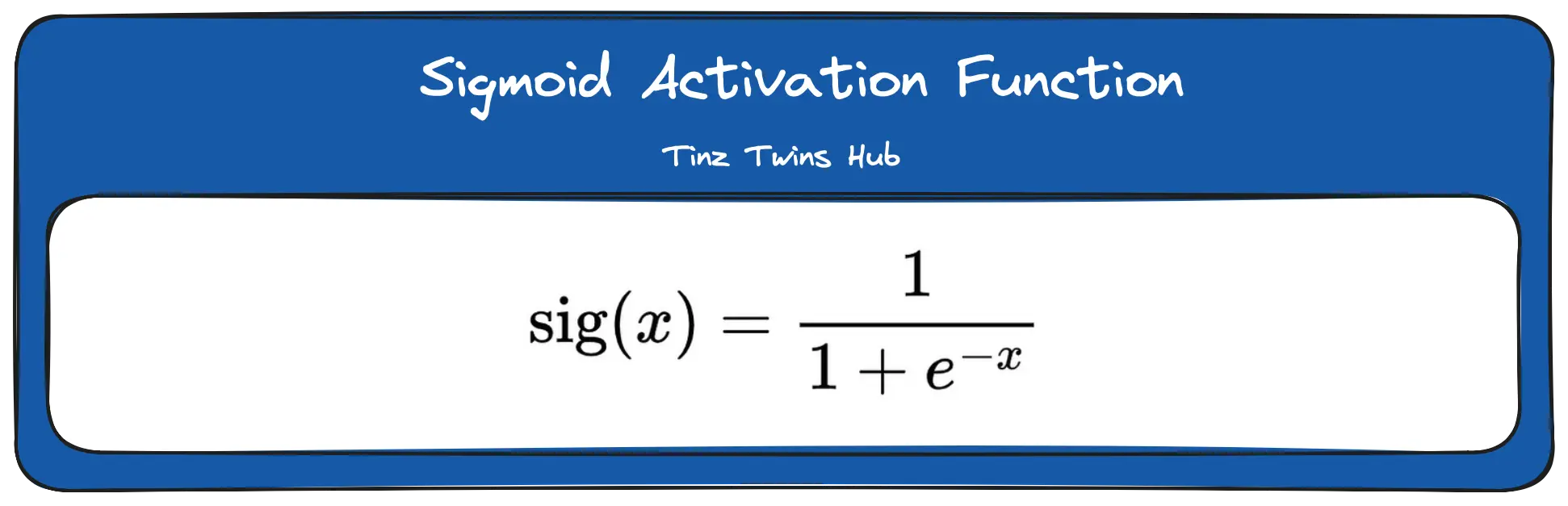
Activation function: The sigmoid activation function has the open interval (0,1) as its value range. Furthermore, the sigmoid function is a bounded and differentiable real function. The formula is:

The derivation is:

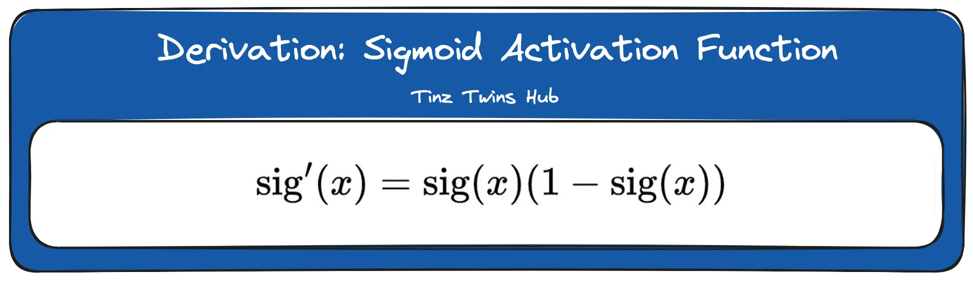
The function sigmoid(z, derivation=FALSE) calculates for a value x the result for the sigmoid or the derivation of the sigmoid.

Cost function: In the function calculate_loss(), we calculate the squared error function. The formula is:

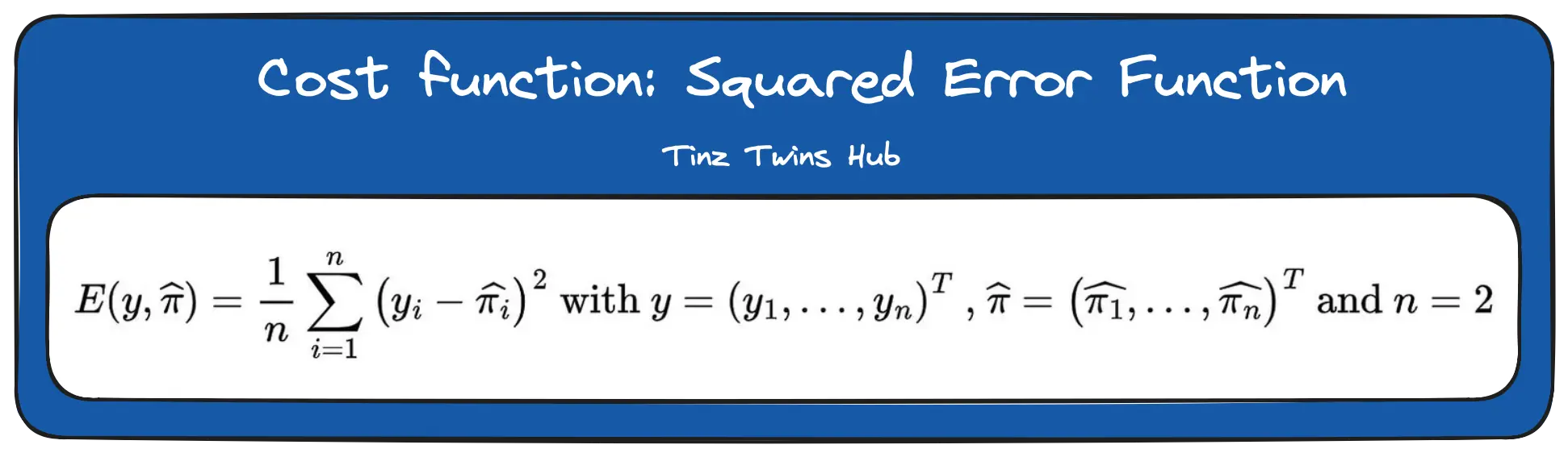
n is the number of classes.

Predict function: In the predict function, we perform feed-forward propagation.

# activation function (sigmod)
def sigmoid(z, derivation = False):
    if derivation:
        return sigmoid(z)*(1-sigmoid(z))
    else:
        return 1/(1+np.exp(-z))

# cost function (Mean squared error function)
def calculate_loss(model, X, y):    
    # extract model parameters
    W1, b1, W2, b2 = model['W1'], model['b1'], model['W2'], model['b2']

    # calculation of the estimated class probabilities
    ## calc hidden layer
    a1 = X.dot(W1) + b1
    h1 = sigmoid(a1)

    ## calc output layer
    a2 = h1.dot(W2) + b2
    probs = sigmoid(a2)[:,0]
    
    # calculation of the cost function value
    cost = np.power(y-probs,2)
    cost = np.sum(cost)/2

    return cost

# predict function
def predict(
        model, 
        x,
        proba = False,
        decision_point = 0.5):
    
    # extract model parameters
    W1, b1, W2, b2 = model['W1'], model['b1'], model['W2'], model['b2']

    # calculation of the estimated class probabilities (Forward Propagation)
    ## calc hidden layer
    a1 = x.dot(W1) + b1
    h1 = sigmoid(a1)

    ## calc output layer
    a2 = h1.dot(W2) + b2
    probs = sigmoid(a2)
    
    if(proba):
        return probs

    return (probs>decision_point)*1

6. Step — Modeling

Now we can design our neural network. We create a network with only one hidden layer. The function build_neural_network() receives as input variables our training data X_train, the labels y_train, the number of gradient descent iterations, the learning_rate, a seed for reproducibility, the number of hidden nodes, and a value for initializing the weights.

We have always written the shape of the array as a comment after the individual lines of code so that you can understand it better. Please go through the code in detail to understand how it works.

def build_neural_network(
        X,                              # features
        y,                              # target
        iterations = 20000,             # number of gradient descent iterations
        learning_rate = 0.1,            # learning rate of Gradient descent
        random_state = None,            # random seed of weights 
        hidden_nodes = 5,               # number of hidden nodes
        rand_range = 0.05):             # initialise the weights

observations = X.shape[0] # number of observations
features = X.shape[1] # number of features

# initialise the parameters to random values:
np.random.seed(random_state)
W1 = np.random.uniform(low = -rand_range, 
                       high = rand_range, 
                       size= (features,hidden_nodes)) # (2,10)
b1 = np.zeros((1,hidden_nodes))   # (1,10)

W2 = np.random.uniform(low = -rand_range, 
                       high = rand_range, 
                       size= (hidden_nodes,1)) # (10, 1)
b2 = np.zeros((1,1))   # (1,1)

# this is what we return at the end
model = {}

# Gradient descent:
for i in range(0, iterations):
    # Forward propagation
    ## calc hidden layer
    a1 = X.dot(W1) + b1   # X: (750, 2), W1: (2,10), a1: (750, 10)
    h1 = sigmoid(a1)   # z1: (750, 10)
    
    ## calc output layer
    a2 = h1.dot(W2) + b2   # z1: (750, 10), W2: (10, 1), a2: (750, 1)
    probs = sigmoid(a2)   # probs: (750, 1)

    # Backpropagation     
    # y.reshape: (750,1), probs: (750, 1), delta1: (750, 1)
    delta1 = (probs-y.reshape((observations,1))) * probs * (1 - probs)   # g(a_k)*(1-g(a_k))*(g(a_k)-t_k^n)
   
    dW2 = np.dot(h1.T, delta1)   # z1.T: (10, 750), delta1: (750,1), dW2: (10,1)
    db2 = np.sum(delta1, axis=0, keepdims=True)  # delta1: (750,1), db2: (1, 1)
    
    delta_j = delta1 * W2.T * h1 * (1 - h1)   # delta1: (750,1), W2.T: (1,10), z1: (750,10), delta_j: (750,10)

    dW1 = np.dot(X.T, delta_j)   # X.T: (2, 750), delta_j: (750,10), dW1: (750,1)
    db1 = np.sum(delta_j, axis=0) # delta_j: (750,10), db1: (10,1)

    # Gradient descent parameter update
    W1 += -learning_rate * dW1  # dW1: (750,1) 
  
    b1 += -learning_rate * db1  # db1: (10,1)
    
    W2 += -learning_rate * dW2
    b2 += -learning_rate * db2
    
    # assign new parameters to the model
    model = { 'W1': W1, 'b1': b1, 'W2': W2, 'b2': b2}
    
    if i % 100 == 0:
        print("Loss after iteration %7d:\t%f" %(i, calculate_loss(model,X,y)))
return model

# Train the neural network
model = build_neural_network(X = X_train,
                    y = y_train, 
                    iterations = 20000,
                    random_state = 4242,
                    hidden_nodes = 5,
                    learning_rate = 0.1,
                    rand_range = 0.1)

7. Step — Evaluation

Classification Report:

from sklearn.metrics import classification_report
predictions = predict(model, X_test)
print(classification_report(y_test, predictions))

# Output
#               precision    recall  f1-score   support
#            0       0.95      0.94      0.94       118
#            1       0.95      0.95      0.95       132
#     accuracy                           0.95       250
#    macro avg       0.95      0.95      0.95       250
# weighted avg       0.95      0.95      0.95       250

The trained neural network has a weighted avg recall and precision of 0.95.

ROC curve with test dataset:

The ROC curve represents the trade-off between the true positive rate (y-axis) and the false positive rate (x-axis). A random classifier lies on the bisector. A bad classifier lies below this line. A classifier becomes better the further it deviates upwards from the bisector. Another criterion for the ROC curve is the area under the ROC curve (AUC) score, where the area under the curve is calculated. A good classifier has an area > 0.5.

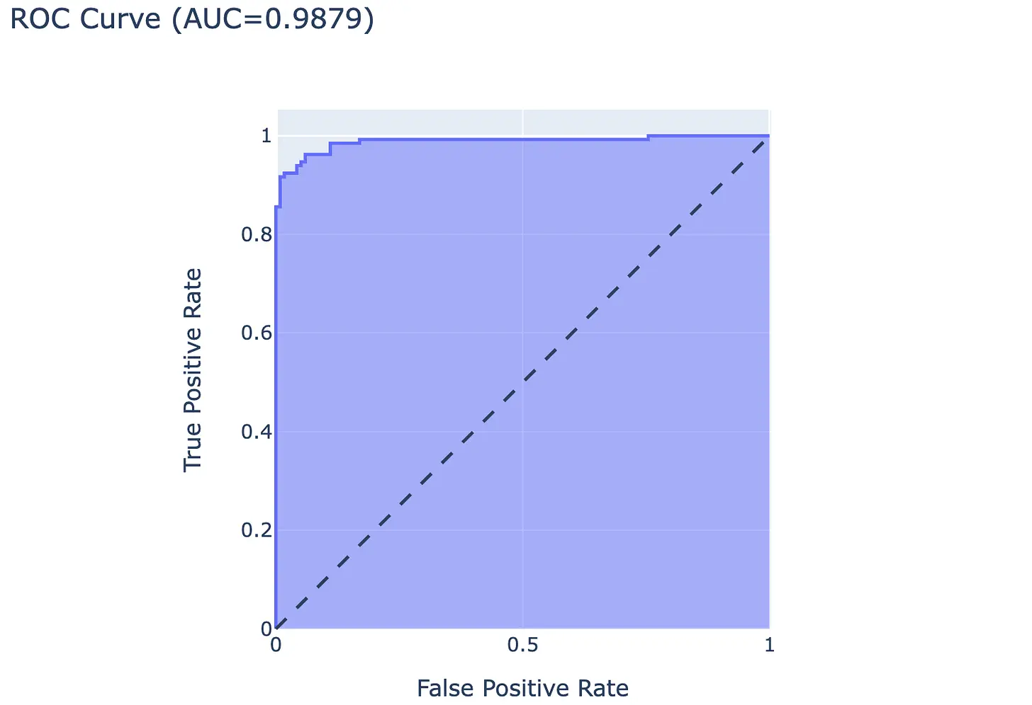
Our neural network has an AUC score of 0.9879.

Experiments

Default Setup for every experiment

• Gradient descent iterations: 10000
• hidden nodes: 5
• learning rate: 0.1

model = build_neural_network(X = X_train,
                    y = y_train, 
                    iterations = 10000,
                    random_state = 4242,
                    hidden_nodes = 5,
                    learning_rate = 0.1,
                    rand_range = 0.1)

1. Change Gradient descent iterations

In the first experiment, we changed the number of gradient descent iterations. So we determine how often the error should be fed back. In Table 1, you can see the results for several runs. We measured the following metrics for the training and test dataset.

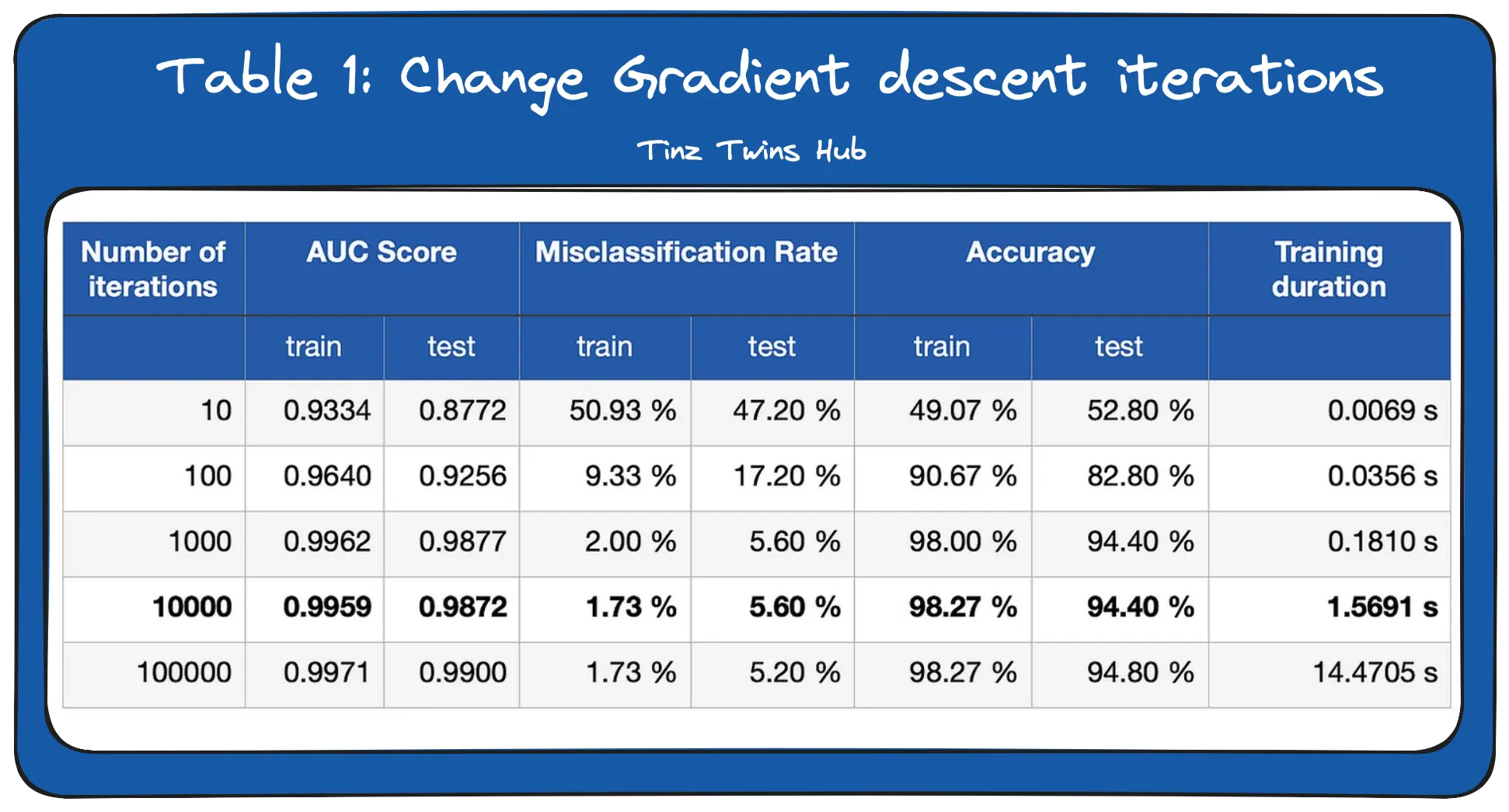
We can see that the AUC score and accuracy increase as we increase the number of iterations. Furthermore, the misclassification rate decreases strongly with an increasing number of iterations. As the number of iterations increases, the weights on the edges of the neural network are updated more and more. The network learns through the weight updates the structures in the training data. But we also see that the performance of the network improves only minimally from 1000 iterations. The more iterations we do, the longer it takes to train the network.

2. Change the number of hidden nodes

In the second experiment, we change the number of nodes in the hidden layer. You can see the results of the experiment in Table 2.

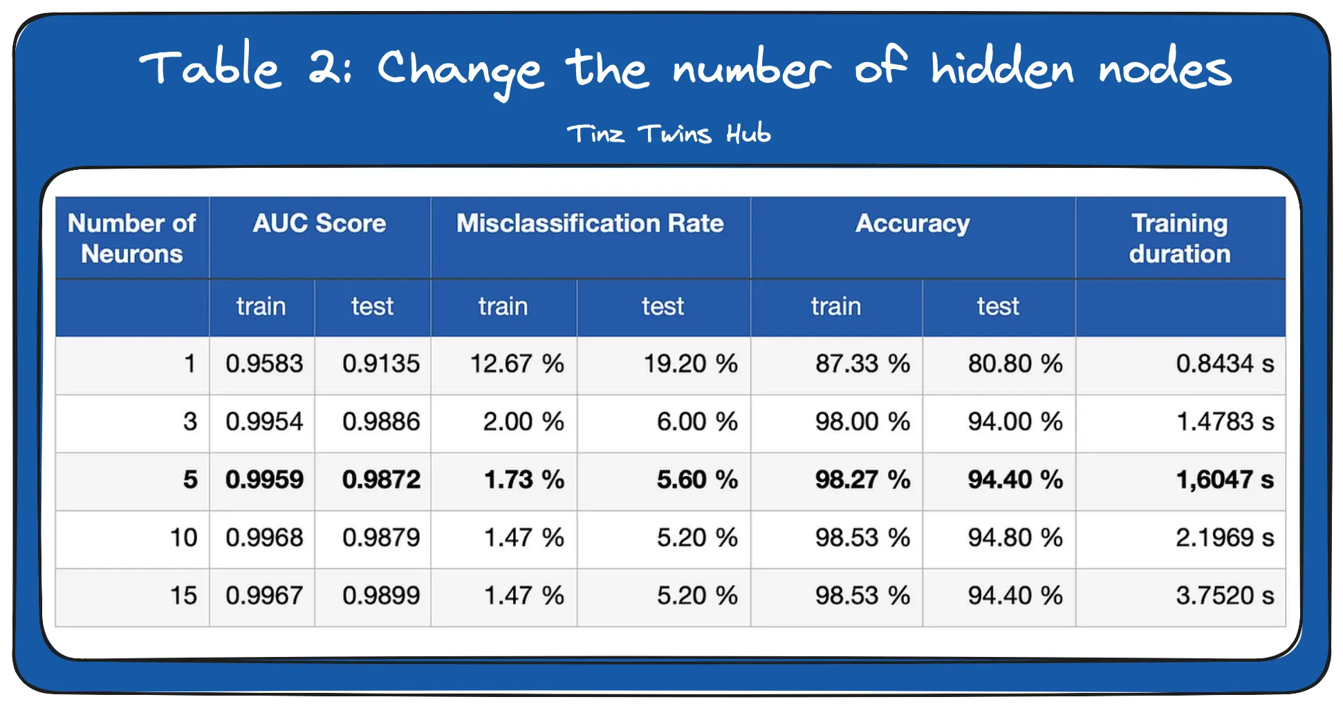
We can see that the network gives good results even with a small number of neurons. The required number of neurons depends on the complexity of the data. For more complex problems, you need more layers with more neurons. The more neurons we use, the longer it takes to train the network.

3. Change the learning rate

In the third experiment, we changed the learning rate. The learning rate specifies how strongly the weights are adjusted.

We see that the learning rate can have a big impact on the performance of the network. With a learning rate of 0.5, the network performed significantly worse. A large learning rate leads to poor results because the neural network does not find the optimal minimum. Finding the optimal learning rate is an art. Furthermore, the learning rate also determines the duration of the training process.

Conclusion

In this article, you have learned how an artificial neural network works. In this context, we have looked at the central concepts in detail. Feedforward describes the flow of input data through the neural network. Backpropagation is used to calculate the error terms per neuron using the gradient descent method.

These concepts also build the basis for more complex network architectures. In addition, you have learned how to implement an artificial neural network from scratch with NumPy. In this context, we looked at the implementation in detail. We also conducted three experiments to see what happens when we change parameters during training.

Thanks so much for reading. Have a great day!

---

💡 Do you enjoy our content and want to read super-detailed articles about data science topics? If so, be sure to check out our premium offer!

Premium Articles

---

References

• KUBAT, Miroslav. An introduction to machine learning. Cham, Switzerland: Springer International Publishing, 2021.
• Hastie, Trevor, et al, The elements of statistical learning: data mining, inference, and prediction (2009). Vol. 2. New York: Springer.
• Dive into Deep Learning (accessed on 17.07.2023)
• A Brief Introduction to Neural Networks (accessed on 17.07.2023)