Mastering Convolutional Neural Networks - A Beginner Guide
Convolutional neural networks (CNNs) have been used in the industry for several years. The flexibility and handling of complex problems are what make CNNs so interesting.

A convolutional neural network belongs to the deep learning methods and is mainly used for the processing of image, video, and audio files. In this context, we speak of deep neural networks. CNNs belong to the subfield of supervised learning.
In this article, we explain how a CNN works. Furthermore, we show you how to implement a CNN with TensorFlow and Keras. We develop a deep learning model for handwriting recognition. In this context, we investigate the limits of a CNN. The central questions of this tutorial are:
- How well can a CNN recognize handwriting?
- Where are the limits of CNNs?
We will conduct a few experiments to investigate the performance of CNNs. Be curious!
CNNs in detail
Structure of a CNN
The following figure illustrates the typical structure of a CNN. A CNN contains several layers. The input images will transform by these layers.
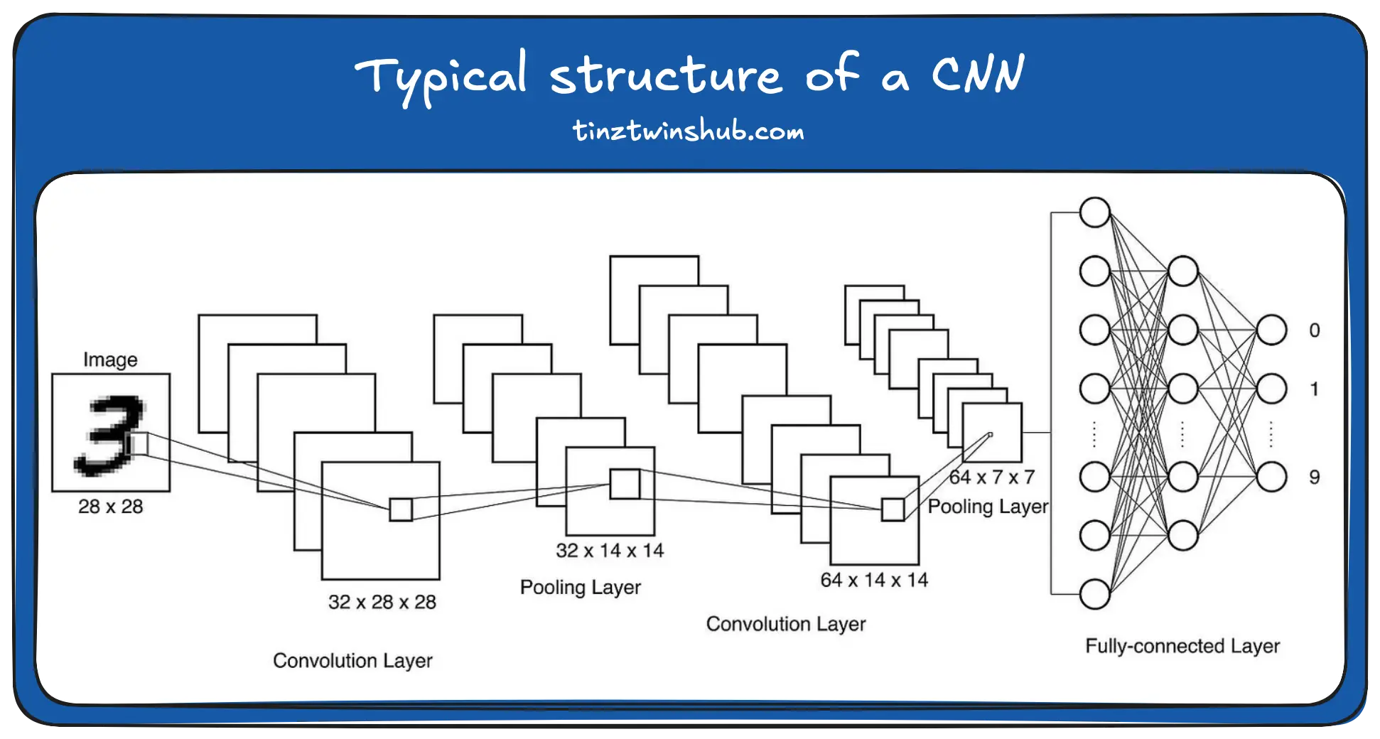
A typical CNN architecture contains Convolutional Layers (Conv-Layers), Pooling Layers (Pool-Layers) and a Fully-connected Layer (FC-Layer). The path of the input data through the CNN is from the Input-Layer to the Output-Layer and is called Feedforward. First, an image passes through a Conv-Layer, which applies several convolution operations to the image. In figure, 32 convolution kernels will apply to the images in the first Conv-Layer.
Then an activation function normalizes the input signals. For CNNs, the ReLu activation function is suitable. The abbreviation stands for rectified linear unit and is defined as ReLu(c) = max(0, c). In the next step, Max-Pooling will apply. A Pool-Layer is usually located between two Conv-Layers to reduce the size of the images by a downsampling operation. This approach reduces the number of model parameters and calculations [1].
Due to max-pooling, CNNs are relatively translation and scaling invariant. In the last step, the data pass through a fully-connected neural network with a classifier (e.g., Softmax). In this example, the classification of handwritten numbers takes place.
Terms of the training process
In this section, we explain the key concepts (in italics) of the training process. During the training of a CNN, the image data will first divide into small packages, the so-called batches. Furthermore, the weights in the convolutional layers will initialize randomly. The CNN finally calculates a classification result for each image in a batch. The calculated result values at the output of the network have an error compared to the true result values.
Then we have to feed the error back into the network. It is also called Backpropagation. The errors will calculate per node. Finally, the gradient descent method will use to minimize the error terms. We speak of a mini-batchgradient descent method when the minimization of the error terms perform for the averaged errors from a batch. In this context, the weights in the convolution kernels will also update.
After all, batches have been processed, a so-called epoch is completed. After each epoch, the images will reshuffle. Then another training process begins. This procedure will repeat until the Data Scientist is satisfied with the result of the CNN.
Dataset
MNIST dataset
We use the Modified National Institute of Standards and Technology (MNIST) dataset for training the model. MNIST is the de facto “Hello World” dataset of computer vision. We can load the dataset directly with Keras.
Our Handwriting dataset
We also use pictures with our handwriting. In the section “Experiments”, we show how well the trained CNN recognizes our handwriting. But how did we create the dataset? First, we wrote the numbers 0 to 9 with a blue pencil on a white sheet of paper. Then we photographed the numbers individually with a camera (iPad Pro: 12 megapixels), cropped them as a square with the macOS preview tool, and saved them.
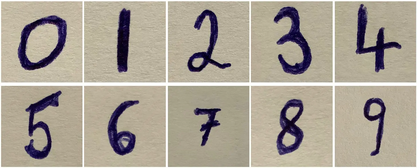
To use our handwriting images, we must transform them into the same form as the MNIST dataset. Three steps are required for this.
Load image:
We read a sample image (number 2) using OpenCV as a greyscale image.
import cv2

img = cv2.imread("imgs/2.jpeg", 0)   # read image

# resize image
dim = (28, 28)   # new image size
img_test = cv2.resize(img, dim, interpolation=cv2.INTER_AREA)
Normalise and show image:
We need to prepare the sample image for the CNN. First we need to normalise the image by dividing the pixels by 255. After this step, we still invert the image because the images from the MNIST dataset are inverted.
import matplotlib.pyplot as plt
%matplotlib inline

img_test = img_test/255
img_test = (img_test-1)*-1
plt.imshow(img_test, cmap="gray_r")
Output:
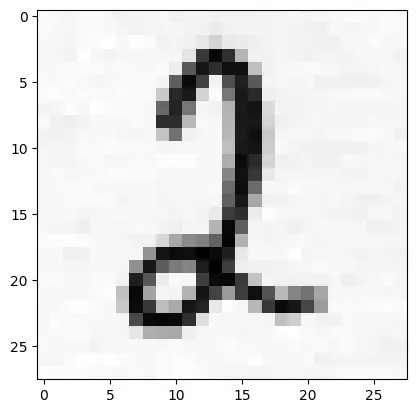
Reshape image:
In addition, we have to add a channel to the images, because we have greyscaled images (1-channel images).
img_test = img_test.reshape(1, 28, 28, 1)
img_test.shape
We use the img_test later for our experiments.
Implementation
1. Step — Technical requirements
You will need the following prerequisites:
- Access to a bash (macOS, Linux, or Windows).
- Installed Python (≥ 3.7)
- A Python package manager of your choice, like conda
- Code editor of your choice (We use VSCode.)
Setup
- Create a conda environment (env):
conda create -n cnn-example python=3.9.12-> Answer the question Proceed ([y]/n)? with y. - Activate the conda env:
conda activate cnn-example - Install the necessary libraries:
pip install tensorflow==2.12.0 matplotlib==3.7.1 opencv-python==4.7.0.72 numpy==1.24.2
2. Step — Imports
from keras.datasets import mnist

import random
import numpy as np
from scipy.ndimage.interpolation import rotate

import matplotlib.pyplot as plt
%matplotlib inline

import cv2
3. Step — Load the MNIST dataset
(x_train, y_train), (x_test, y_test) = mnist.load_data()
4. Step — Preprocessing labels
# save labels as "one hot encoded"
from keras.utils.np_utils import to_categorical
y_cat_test = to_categorical(y_test,10)
y_cat_train = to_categorical(y_train,10)
5. Step — Preprocessing: Normalise the MNIST dataset
x_train = x_train/255
x_test = x_test/255
6. Step — Transform the MNIST dataset
The MNIST dataset has 60.000 images with 28 x 28 pixels. We have to add a channel to the images, because we have greyscaled images (1-channel images).
x_train = x_train.reshape(x_train.shape[0], 28, 28, 1)
x_test = x_test.reshape(x_test.shape[0],28,28,1)
7. Step — Define CNN Model
We design a CNN model using Tensorflow and Keras for the MNIST dataset. The network has three convolutional layers with Max-Pooling. The first convolutional layer has 32 filters with a kernel-
size of 3x3 and ReLu as an activation function. The other two Conv-Layers have 64 filters with a kernel size of 3x3 and also the ReLu function as an activation function. We use the Adam optimizer and the cross entropy as the loss function.
from keras.models import Sequential
from keras.layers import Dense, Conv2D, MaxPool2D, Flatten

model = Sequential()

model.add(Conv2D(filters=32, kernel_size=(3,3),input_shape=(28, 28, 1), activation='relu',))
model.add(MaxPool2D(pool_size=(2, 2)))

model.add(Conv2D(filters=64, kernel_size=(3,3), activation='relu',))
model.add(MaxPool2D(pool_size=(2, 2)))

model.add(Conv2D(filters=64, kernel_size=(3,3), activation='relu',))
model.add(Flatten())

model.add(Dense(128, activation='relu'))
model.add(Dense(10, activation='softmax'))

model.compile(loss='categorical_crossentropy',
              optimizer='adam',
              metrics=['accuracy'])
model.summary()

# Output
# Model: "sequential"
# _________________________________________________________________
#  Layer (type)                Output Shape              Param #
# =================================================================
#  conv2d (Conv2D)             (None, 26, 26, 32)        320

#  max_pooling2d (MaxPooling2D  (None, 13, 13, 32)       0
#  )

#  conv2d_1 (Conv2D)           (None, 11, 11, 64)        18496

#  max_pooling2d_1 (MaxPooling  (None, 5, 5, 64)         0
#  2D)

#  conv2d_2 (Conv2D)           (None, 3, 3, 64)          36928

#  flatten (Flatten)           (None, 576)               0

#  dense (Dense)               (None, 128)               73856

#  dense_1 (Dense)             (None, 10)                1290

# =================================================================
# Total params: 130,890
# Trainable params: 130,890
# Non-trainable params: 0
# _________________________________________________________________
8. Step — Training
model.fit(x_train, y_cat_train, epochs=10, batch_size=64)
9. Step — Evaluation
model.evaluate(x_test,y_cat_test)

# Output
# [0.03408227860927582, 0.9915000200271606]

from sklearn.metrics import classification_report
import numpy as np

predictions = np.argmax(model.predict(x_test), axis=-1)
print(classification_report(y_test,predictions))

# Output
#               precision    recall  f1-score   support
#            0       1.00      1.00      1.00       980
#            1       0.99      1.00      1.00      1135
#            2       0.99      0.99      0.99      1032
#            3       0.98      1.00      0.99      1010
#            4       0.99      1.00      0.99       982
#            5       1.00      0.98      0.99       892
#            6       1.00      0.98      0.99       958
#            7       0.99      0.99      0.99      1028
#            8       0.99      0.99      0.99       974
#            9       0.99      0.99      0.99      1009
#     accuracy                           0.99     10000
#    macro avg       0.99      0.99      0.99     10000
# weighted avg       0.99      0.99      0.99     10000
We see that the trained model has an accuracy of 99% on the test dataset.
Experiments
1. Experiment: Predict our handwriting numbers
pred = model.predict(img_test)
pred_number = np.argmax(pred)

print("Number: " + str(pred_number))
pred_prob = np.amax(pred)
print("Accuracy: " + str(pred_prob*100) + " %")

# Output
# Number: 2
# Accuracy: 99.98 %
Now we can test the trained network with pictures of our handwriting. The numbers 0 to 9 were correctly classified by the network. For example, the number 2 has an accuracy of 99.98 %.
2. Experiment: Predict our rotated handwriting numbers
Research Question 1: What happens if you turn the digits 90 (to the left and right) or 180 degrees?
Proposition: “The trained network misclassifies a rotated digit, whereas the numbers 0, 1 and 8 are correctly classified when rotated by 180 degrees”.
We tested the trained network with rotated images of the number 8. First, we rotated the number by 90 degrees. Here, the CNN classified a 6 with an accuracy of approx. 29%. When rotated by 180 degrees, CNN correctly classified the number 8 with an accuracy of 99.34%. Then we tried out the number 2. We found that CNN correctly classified the number 2 at a rotation of 90 degrees with an accuracy of 44.23%. Further, the CNN incorrectly classifies the number 2 at a rotation of 180 degrees.
The numbers 0, 1, and 8 are correctly classified when rotated by 180 degrees. You get the number itself again with a rotation of 180 degrees. Furthermore, the numbers 6 and 9 will reverse in a rotation of 180 degrees.
Is there a solution to the problem?
Solution 1: A possible solution would be to rotate the images into the correct orientation before predicting. A realization of this approach shows the work of Daniel Saez [2]. The author proposes to train a CNN that predicts the rotation angle of an image. The predicted rotation angle will use to bring the image into the correct orientation. In the next step, CNN predicts the rotated numbers. This solution is very time-consuming.
Solution 2: Another solution would be that we additionally train the CNN with rotated images (90 degrees, -90 degrees, 180 degrees).
So we randomly rotate the images in the MNIST dataset by 90, -90 and 180 degrees. Then we trained the CNN with the original and rotated images.
The Classification Report of the new model:
model.evaluate(x_test,y_cat_test)

# Output
# [0.07178938388824463, 0.9797499775886536]

from sklearn.metrics import classification_report
import numpy as np

predictions = np.argmax(model.predict(x_test), axis=-1)
print(classification_report(y_test,predictions))

# Output
#               precision    recall  f1-score   support
#            0       1.00      0.99      0.99      1960
#            1       0.99      1.00      0.99      2270
#            2       0.99      0.97      0.98      2064
#            3       0.98      0.99      0.98      2020
#            4       0.98      0.98      0.98      1964
#            5       0.98      0.98      0.98      1784
#            6       0.97      0.96      0.96      1916
#            7       0.97      0.98      0.97      2056
#            8       0.99      0.99      0.99      1948
#            9       0.96      0.96      0.96      2018
#     accuracy                           0.98     20000
#    macro avg       0.98      0.98      0.98     20000
# weighted avg       0.98      0.98      0.98     20000
The report shows that the new model is still very good.
The new model correctly classified the number 2 (90 degrees rotated) with an accuracy of 99.95%. Furthermore, the model correctly classified the number 2 (180 degrees rotated) with an accuracy of 93.09%. Furthermore, the number 2 (-90 degrees rotated) has an accuracy of 90.88%.
The new model correctly classifies rotated numbers with an accuracy of over 90%.
Conclusion
In this article, we have explained how a CNN works. We also designed a CNN with TensorFlow and Keras. We then used CNN to conduct experiments. In the first experiment, we tried to recognize our handwriting. CNN classified our handwriting very well. The second experiment showed that a CNN with rotated numbers does not work. To solve the problem, we presented two proposed solutions. CNNs are relatively translation and scaling invariant but not truly rotation invariant.
Thanks so much for reading. Have a great day!
References
- [1] Cs231n: Convolutional neural networks for visual recognition. https://cs231n.github.io/convolutional-networks/.
- [2] https://d4nst.github.io/2017/01/12/image-orientation/
- [3] Zafar, I., Tzanidou, G., Burton, R., Patel, N. and Araujo, L., 2018. Hands-on convolutional neural networks with TensorFlow: Solve computer vision problems with modeling in TensorFlow and Python. Packt Publishing Ltd.
- [4] Hands-On Computer Vision with TensorFlow 2: Leverage deep learning to create powerful image processing apps with TensorFlow 2.0 and Keras
