**The bootstrap method is a resampling technique in which one draws many samples again from one sample. It is used to estimate summary statistics like the mean or standard deviation.**
Photo by Javier Quesada on Unsplash
The bootstrap method is a powerful statistical tool, and it is useful for small samples. The advantage of the bootstrap method is that this method does not make any distribution assumptions. It is a non-parametric method and can also be used when normal distribution assumptions of the model are not applicable.
## How does bootstrapping work?
The bootstrap method works as follows:
* Take k samples with replacement from a given dataset.
* For each sample, calculate the statistic/parameter you are interested in.
* You get k different estimates for a given statistic/parameter. You can then use these estimates to calculate a confidence interval for the statistic.
There is a [YouTube video by Andy Field](https://www.youtube.com/watch?v=LZtPDgoskfI){:target="_blank" rel="noopener"} in which he explains bootstrapping clearly. From minute 27:27, he talks about bootstrapping. However, the video is not suitable for everyone, as Andy Field explains the topic in a very humorous way.
## Bootstrapping and the central limit theorem
The central limit theorem is a fundamental theorem of statistics. The central limit theorem states that the mean and sum of many independent identically distributed random variables are approximately normally distributed.
Sounds complicated? The bootstrap method makes the central limit theorem easy to understand. We want to illustrate this with an example.
There are many ways to implement the bootstrap method in Python. The easiest way is to use the `bootstrap()` function from the [SciPy](https://pypi.org/project/scipy/){:target="_blank" rel="noopener"} package.
First, we import the necessary Python packages.
```python
import numpy as np
import seaborn as sns
import matplotlib.pyplot as plt
from scipy.stats import bootstrap
```
We import the following libraries:
* [**numpy**](https://numpy.org/doc/stable/index.html){:target="_blank" rel="noopener"}: The library is the basic package for scientific computing in Python.
* [**seaborn**](https://seaborn.pydata.org/){:target="_blank" rel="noopener"}: This library provides a high-level interface for creating stunning graphics.
* [**matplotlib**](https://matplotlib.org/stable/index.html){:target="_blank" rel="noopener"}: With this library, you can create different visualizations.
* [**scipy.stats**](https://docs.scipy.org/doc/scipy/reference/stats.html){:target="_blank" rel="noopener"}: This module contains several functions from statistics. We only use the bootstrap function.
Now, we look at data from an exponential distribution.
```python
X = np.random.exponential(scale=1, size=10000)
mean_value = np.mean(X)
print(mean_value)
# Output:
# 0.9971608985989188
```
**Function parameters of** `np.random.exponential()`**:**
* **scale**: Scale factor beta
* **size**: Output shape (we choose 10,000 values)
First, we use `np.random.exponential()` to create a dataset `X` that is exponentially distributed. The formula for the probability density function is:
Formula: Probability density function (see numpy reference)
The mean value of the exponential distribution is approximately **0.9972**.
Now, let’s take a visual look at the data. We create a density plot in Python.
```python
ax = sns.distplot(X)
ax.set(xlabel='X', ylabel='Density', title='Exponential distribution plot')
```
For the density plot, we use the Seaborn Library.
**Density Plot:**
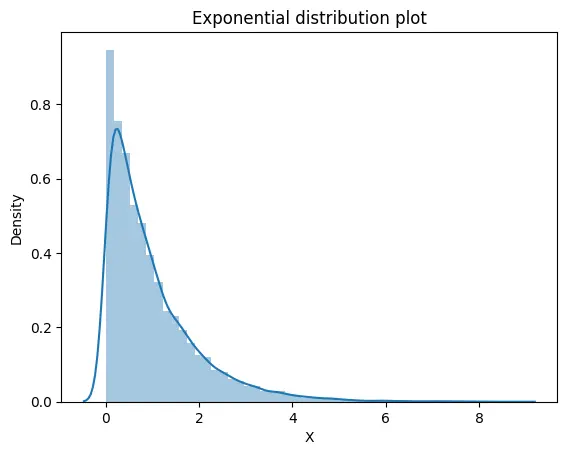
We can see that the data are not normally distributed. Now we will use the bootstrap method to estimate the mean of the distribution.
Before performing the bootstrap procedure, you have to choose two parameters:
* **Size of the sample**
* **Number of repetitions**
We chose a sample size of 100. In addition, we execute two bootstrap experiments.
```python
dataset_choice = np.random.choice(X, size=100)
```
**First Experiment:**
In the first experiment, we performed **50 bootstrap repetitions**.
```python
dataset = (dataset_choice,)
res = bootstrap(dataset, np.mean, n_resamples=50, random_state=42)
ax = sns.histplot(res.bootstrap_distribution)
plt.axvline(x=dataset_choice.mean(), linewidth=3, color='red', label="mean", alpha=0.5)
plt.text(x=1.1, y=13, s=round(dataset_choice.mean(), 2))
plt.legend(["mean"])
ax.set(xlabel='Means', ylabel='Frequency', title='Histogram: Mean values - 50 bootstrap replicated datasets')
```
**Output:**
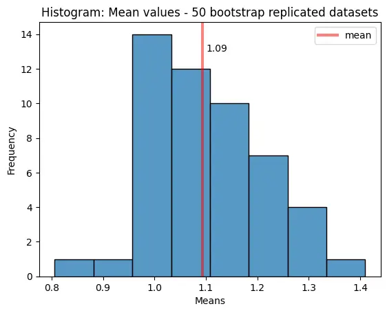
We see that the distribution is different from an exponential distribution. It is more like a normal distribution. The 50 bootstrap replicated datasets have a mean value of **1.09**.
**Second Experiment:**
The second experiment contains **1,000 bootstrap repetitions**.
```python
dataset = (dataset_choice,)
res = bootstrap(dataset, np.mean, n_resamples=1000, random_state=42)
ax = sns.histplot(res.bootstrap_distribution)
plt.axvline(x=dataset_choice.mean(), linewidth=3, color='red', label="mean", alpha=0.5)
plt.text(x=1.06, y=121, s=round(dataset_choice.mean(), 2))
plt.legend(["mean"])
ax.set(xlabel='Means', ylabel='Frequency', title='Histogram: Mean values - 1000 bootstrap replicated datasets')
```
**Output:**
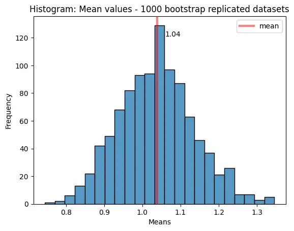
Now we see even more clearly that it is a normal distribution. The mean value of the bootstrap replicated datasets is **1.04**.
The mean of the original dataset was approximately **0.9971**. The bootstrap mean is **1.09 (50 repetitions)** and **1.04 (1,000 repetitions)**. We have to keep in mind that we only used a sample of 100 values for the bootstrap method. So using the bootstrap method, we can make a good estimate of statistical parameters. In our example, we know the distribution of the population. However, this is often not the case. The bootstrap method gives us a good estimate of different distribution parameters.
Thanks so much for reading. **Have a great day!**
💡 Do you enjoy our content and want to read super-detailed guides about AI Engineering? If so, be sure to check out our premium offer!