Mastering Bollinger Bands - A Comprehensive Guide with Python and OpenBB
Have you ever watched the ups and downs of the stock market and wondered how you can predict the next move? Bollinger Bands, a tool to visualize volatility, could help you understand trading better.

Traders often look for landmarks in charts. The Bollinger Bands are a popular method to find such landmarks in charts. They are used in technical analysis and serve as volatility indicators.
You can use this method for forecasting share price reversals. The indicator is based on a rolling mean and the standard deviation of the rolling mean. That may sound complicated at first glance! Don’t panic - you’ll understand after reading this article.
In this article, we explain the idea of Bollinger Bands and how you can calculate them. In addition, we apply the Bollinger Bands to the Tesla stock using Python and OpenBB. OpenBB simplifies the calculation of the Bollinger Bands.
Ready to learn more? Let’s dive in.
Idea and Interpretation
The Bollinger Bands are parallel bands running through the chart of a stock. For a better understanding, let’s take a look at an example. In the following, you see the Tesla stock with marked Bollinger Bands. We created this chart with Python. You’ll learn more about that later in this article.
First, you must understand how the Bollinger Bands work.
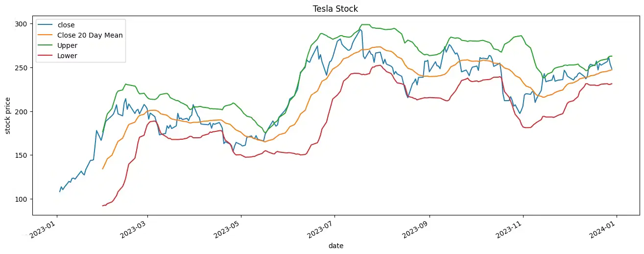
Bollinger Bands consist of three lines.
- The middle band is a rolling mean.
- The upper band is two standard deviations above the rolling mean.
- The lower band is two standard deviations below the rolling mean.
Look at the chart above. You notice that the share price mostly moves within the Bollinger Bands. Furthermore, the Bollinger Bands don’t start on January 1, 2023. That’s because they are based on the rolling mean. You’ll learn more about that later in this article.
But how can we use the indicator to draw possible conclusions for predictions? We can use the Bollinger Bands to measure the volatility of a stock. The width of the Bollinger Bands indicates the volatility of the price. The direction of the Bollinger Bands provides information about the direction of the price.
Technically, the price is relatively high when it breaks out of the Bollinger Bands. At this point, it is better not to buy shares. That makes a correction with falling prices more likely. On the other hand, prices are relatively low when the price is below the lower band. At this point, the shares are valued low. It might be worth buying shares.
If the upper and lower bands are moving closer together, a significant price change is more likely, but its direction isn’t clear.
The Bollinger Bands, as a standalone instrument, don’t generate buy or sell signals. They can help traders or investors find potential turning points. You can’t predict share prices one hundred percent. Always be aware of that!
Practical example with Python and OpenBB
In this section, we demonstrate how to create Bollinger Bands using Python and OpenBB. You can read our article “Every Investor is talking about OpenBB: Here’s why?” if you want to learn more about OpenBB.
As an example, we use the stock market data of Tesla. Tesla stock has been very volatile in the last few years, so it’s a perfect example for this article.
Load Tesla’s stock market data
In the first step, we import the OpenBB Python package. The OpenBB package gives you access to a lot of financial data.
from openbb import obb
After that, we load the stock data of Tesla with a single function call. We load the data for the year 2023 with an interval of one day. As a data provider, we use yfinance. Look at the following code:
df_daily = obb.equity.price.historical(symbol="tsla",
                                       start_date="2023-01-01",
                                       end_date="2023-12-31",
                                       interval="1d",
                                       provider="yfinance",
                                       adjusted=True).to_df()
df_daily.drop(['dividends', 'stock_splits'], axis=1, inplace=True)

df_daily.head()

# Output
#	              open	 high	   low	 close	   volume
#       date
# 2023-01-03	118.47	118.80	104.64	108.10	231402800
# 2023-01-04	109.11	114.59	107.52	113.64	180389000
# 2023-01-05	110.51	111.75	107.16	110.34	157986300
# 2023-01-06	103.00	114.39	101.81	113.06	220911100
# 2023-01-09	118.96	123.52	117.11	119.77	190284000
After loading the data, we remove the columns ‘dividends’ and ‘stock_splits’ because we don’t need them in the further tutorial.
Great! We have loaded Tesla’s stock market data. Next, we can calculate the rolling mean.
Calculate the rolling mean in Python
Before we calculate the rolling mean, it’s always a good idea to plot the data so you can get a basic understanding of the data.
Let’s plot the data!
df_daily['close'].plot(xlabel='date',
                        ylabel='stock price',
                        title = "Tesla Stock",
                        figsize=(16,6))
Output:
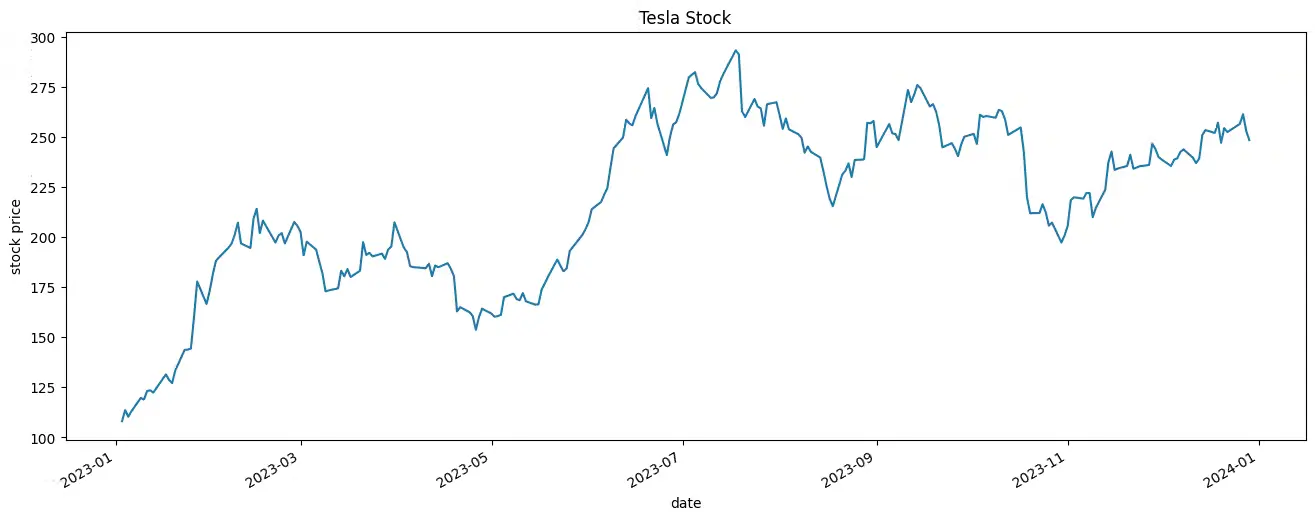
You see that the Tesla stock had a positive trend in 2023. But we also see some stock setbacks.
Great! Let’s calculate the rolling mean.
df_daily.rolling(window=4).mean().head()

# Output
#	                open	    high	     low	   close	     volume
#       date
# 2023-01-03	     NaN	     NaN	     NaN	     NaN	        NaN
# 2023-01-04	     NaN	     NaN	     NaN	     NaN	        NaN
# 2023-01-05	     NaN	     NaN	     NaN	     NaN	        NaN
# 2023-01-06	110.2725	114.8825	105.2825	111.2850	197672300.0
# 2023-01-09	110.3950	116.0625	108.4000	114.2025	187392600.0
You see that the first three rows have NaN values. That’s why we set our window to 4. The calculation is simple. Now, the cell (2023-01-06 / open) contains the value 110.2725.
If we calculate the average of the first four values in the “open” column, we get the value 110.2725. Look up the values in the output further up in this article. The calculation is as follows:
(118.47 + 109.11 + 110.51 + 103.00)/4 = 110.2725
That’s how the rolling mean works.
Next, we can calculate the 20-day rolling mean for the Tesla stock. We can do this with the following Python code.
df_daily['Close: 20 Day Mean'] = df_daily['close'].rolling(window=20).mean()
df_daily[['close', 'Close: 20 Day Mean']].plot(xlabel='date',
                                                ylabel='stock price',
                                                title = "Tesla Stock",
                                                figsize=(16,6))
Output:
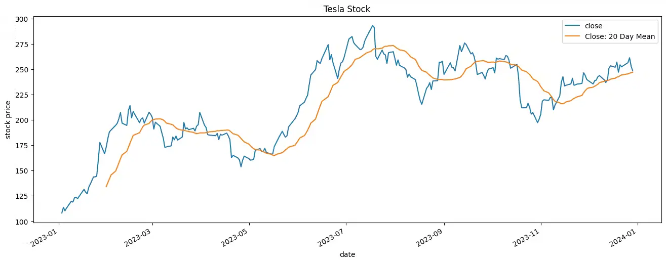
What do you notice? You can see that we don’t have a rolling mean for the first days of the chart. That is due to the calculation of the rolling mean, as we discussed above.
The rolling mean is the middle line of the Bollinger Bands. The following section deals with the calculation of the upper and lower bands.
Create Bollinger Bands in Python
You can create the upper and lower bands easily with Python. First, we calculate the 20-day rolling mean and add the results to our dataframe df_daily with the column name ‘Close 20 Day Mean’.
In the next step, we calculate the upper band by adding twice the standard deviation to the 20-day rolling mean. In addition, we calculate the lower band by subtracting twice the standard deviation from the 20-day rolling mean. The Python code looks as follows:
# Close 20 Rolling Mean (RM)
df_daily['Close 20 Day Mean'] = df_daily['close'].rolling(window=20).mean()

# Upper = 20 RM + 2*Std(20)
df_daily['Upper'] = df_daily['Close 20 Day Mean'] + 2 * df_daily['close'].rolling(window=20).std()

# Lower = 20 RM - 2*Std(20)
df_daily['Lower'] = df_daily['Close 20 Day Mean'] - 2 * df_daily['close'].rolling(window=20).std()
We added the three bands to our dataframe, so we can now easily plot them.
df_daily[['close', 'Close 20 Day Mean', 'Upper', 'Lower']].plot(xlabel='date',
                                                                ylabel='stock price',
                                                                title = "Tesla Stock",
                                                                figsize=(16,6))
Output:

Now, you see the plot that we showed you at the beginning of the article. Next, we will look at the automatic calculation with OpenBB.
Create Bollinger Bands with OpenBB
With OpenBB, you can calculate the Bollinger Bands using just one command. In the following Python code, we use the obb.technical.bbands(...) method to calculate the three Bollinger Bands lines. We pass our data (df_daily), the target column ('close'), the standard deviation (2), and the rolling mean method ('sma') as parameters. 'sma' stands for Simple Moving Average.
results = obb.technical.bbands(data=df_daily, target='close', length=20, std=2, mamode='sma').to_df()
The function returns an object in the form of an OBBject. We convert this object into a dataframe by using .to_df(). We obtain results as a dataframe.
In the next step, we plot the Bollinger Bands with the following Python Code.
results[['close', 'close_BBM_20_2.0', 'close_BBU_20_2.0', 'close_BBL_20_2.0']].plot(xlabel='date',
                                                                                    ylabel='stock price',
                                                                                    title = "Tesla Stock",
                                                                                    figsize=(16,6))
Output:
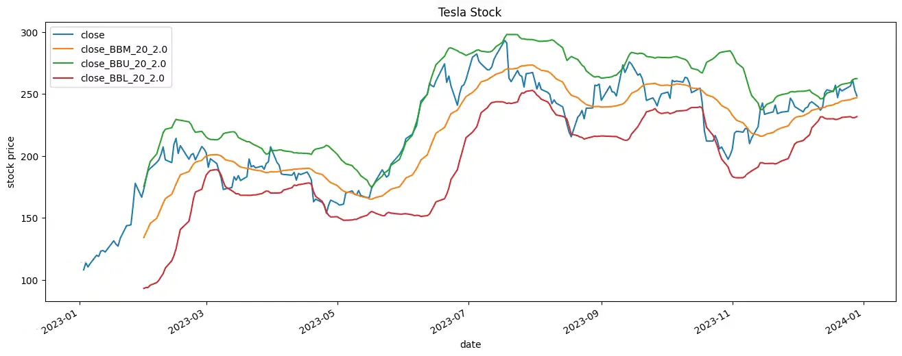
We get the same result as in the Python example before. Perfect, now you can use Bollinger Bands for your own examples.
Conclusion
The Bollinger Bands indicator is a popular technical analysis tool that delivers insights into stock price movements and volatility. You can use Python and OpenBB to calculate the Bollinger Bands. That can help you make better trading decisions. It’s important to use the Bollinger Bands alongside other indicators and analysis methods to improve trading strategies and minimize risk.
Thanks so much for reading. Have a great day!
Disclaimer: All texts, notes and information provided by tinztwins do not constitute investment advice or a recommendation to buy or sell securities. They are for personal information only and reflect the opinion of the authors. No recommendation for a specific investment strategy is given.


