Time Shifting in Pandas using the time series data from Tesla stock

In the fast-paced world of stock trading, analyzing time series data is crucial for making informed decisions. With the help of advanced tools like Pandas, analyzing time series data has become more straightforward.

Generated with Microsoft Copilot

Imagine you need to shift all rows in a DataFrame, a common task in time series analysis. For certain Machine Learning (ML) models, it’s necessary to shift the time series data by a specific number of steps. The Pandas Library excels at this task.

In this article, we look at examples to show how the Pandas shift function works. We’ll use Tesla stock’s time series data as our example dataset.

We’ll cover the following points:

• Technical requirements
• Load time series data with OpenBB
• Time Shifting in Pandas

Technical requirements

For this tutorial, you should be familiar with the Python programming language. If you are not familiar with Python or would like to improve your data science skills, take a look at our online course recommendations.

Prerequisites

• Python package manager of your choice like conda.
• A code editor of your choice like Visual Studio Code.

Setup

• Create a conda environment (env): conda create -n openbb-env python=3.11.7 -> Answer the question Proceed ([y]/n)? with y.
• Activate the conda env: conda activate openbb-env
• Install openbb: pip install openbb

Load time series data with OpenBB

We use OpenBB to get Tesla’s stock market data. If you’re not familiar with OpenBB, you might want to check out our article. First, we need to import the openbb package. After that, we can get Tesla’s historical stock data by using obb.equity.price.historical(). That gives us past prices of the stock, including the opening, highest, closing prices, and the volume of stocks traded.

The function works with different parameters depending on where the data comes from. In our case, we’re using the yfinance data provider. For more information, look at the OpenBB documentation. We also set the symbol="tsla", the start and end dates, choose an interval="1d", and turn on adjusted=True.

The adjusted parameter is important because things like stock splits and dividends can change the stock’s price. To correctly compare share prices over time, we need to adjust the prices for these events. This adjustment ensures that the prices are corrected based on the date an event changed the price.

df_daily = obb.equity.price.historical(symbol="tsla", 
                                       start_date="2023-01-01", 
                                       end_date="2023-12-31", 
                                       interval="1d", 
                                       provider="yfinance", 
                                       adjusted=True).to_df()

# We remove the columns 'dividends' and 'stock_spilts' 
# because we no longer need them in this article.
df_daily.drop(['dividends', 'stock_splits'], axis=1, inplace=True)

df_daily.head()

Output:

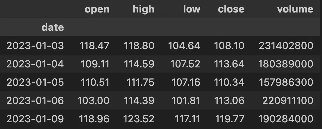
You might wonder why the first date is 03.01.2023 and not 02.01.2023 on a Monday. As you might know, stock exchanges are open only on weekdays. On 02.01.2023, the stock exchanges like Wall Street and Nasdaq were closed to make up the New Year’s Day. That is why the time series begins on 03.01.2023.

Next, we can use the tail() function to see the last five rows. We’ll need this information later to compare these rows with those we get after performing the time shifting.

df_daily.tail()

Output:

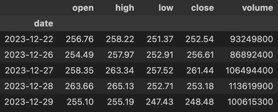
In the output, we see the stock prices and the volume for the last days of 2023. December 29, 2023, was a Friday and the last trading day of the year.

---

---

Time Shifting in Pandas

We use the shift() function of the Pandas Package for time shifting. The shift() function has the following parameters:

df_daily.shift(periods=1, freq=None, axis=0, fill_value=_NoDefault.no_default)

Let’s quickly go over the parameters.

• periods: Number of periods to shift. It can be either positive or negative.

• freq: Frequency-based shifting. The DataFrame’s index must be a date or datetime; otherwise, an error will occur.

• axis: Shift direction (Default=0).

• fill_value: You can select the fill value, such as 0.

For more details on the function, you can refer to the pandas documentation.

Shifting time series with periods

We can move the time series forward or backward by a specific number of periods using the periods parameter. In the example below, we set periods=1, which means we shift the time series forward by one day.

df_daily.shift(periods=1)

Result:

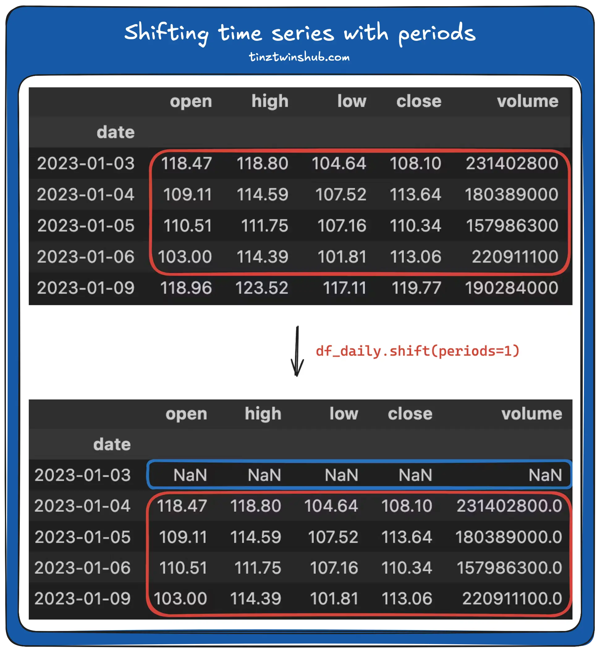
The row values are shifted forward by one day (marked red), and the first row now contains NaN (marked blue). By default, missing values are filled with NaN.

Next, let’s use the parameter periods=-1. This setting shifts the time series in the opposite direction. Here’s the code to do that:

df_daily.shift(periods=-1)

Result:

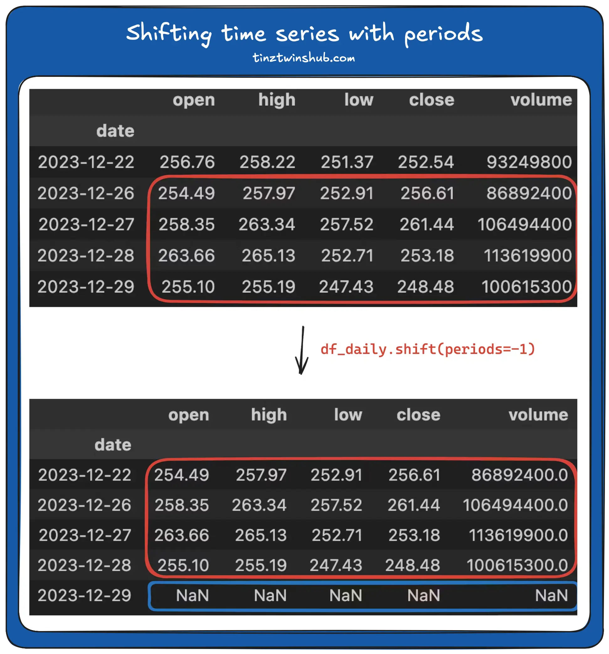
Now, the last row of our dataset has NaN values because we moved the time series one day back. However, we can decide what to fill these missing values with. For example, we can replace all missing values with 0.

df_daily.shift(periods=1, fill_value=0)

Result:

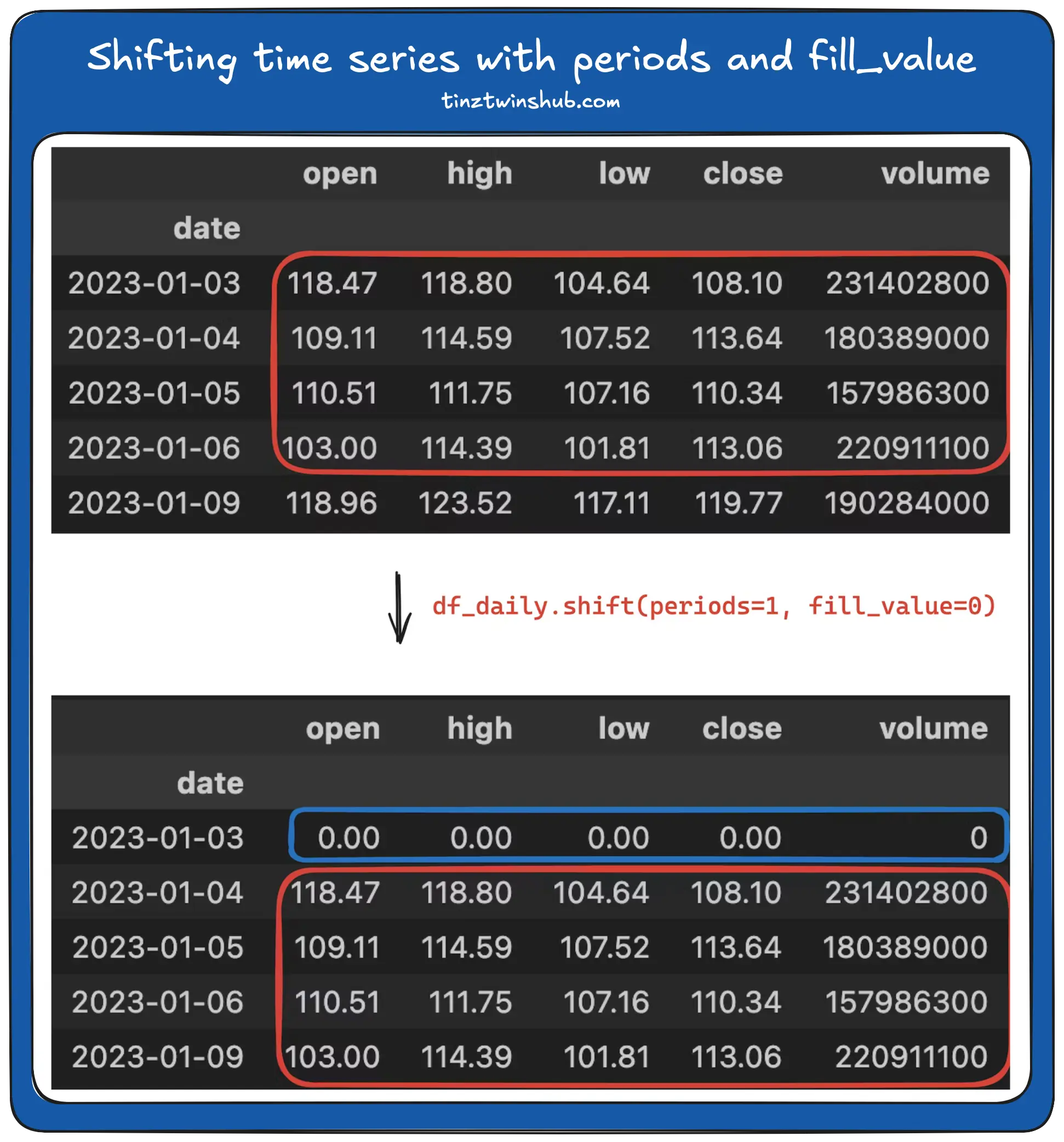
You can see that the missing values have been replaced with 0.

Shifting time series with freq

The freq parameter lets you shift the time series based on frequency. In this scenario, we shift the index. That is very useful for time series data. In the example below, we shift the index by three days. This means the time series then starts on 06.01.2023 and ends on 01.01.2024.

df_daily.shift(freq='3D')

Equivalent:

df_daily.shift(periods=3, freq='D')

Result:

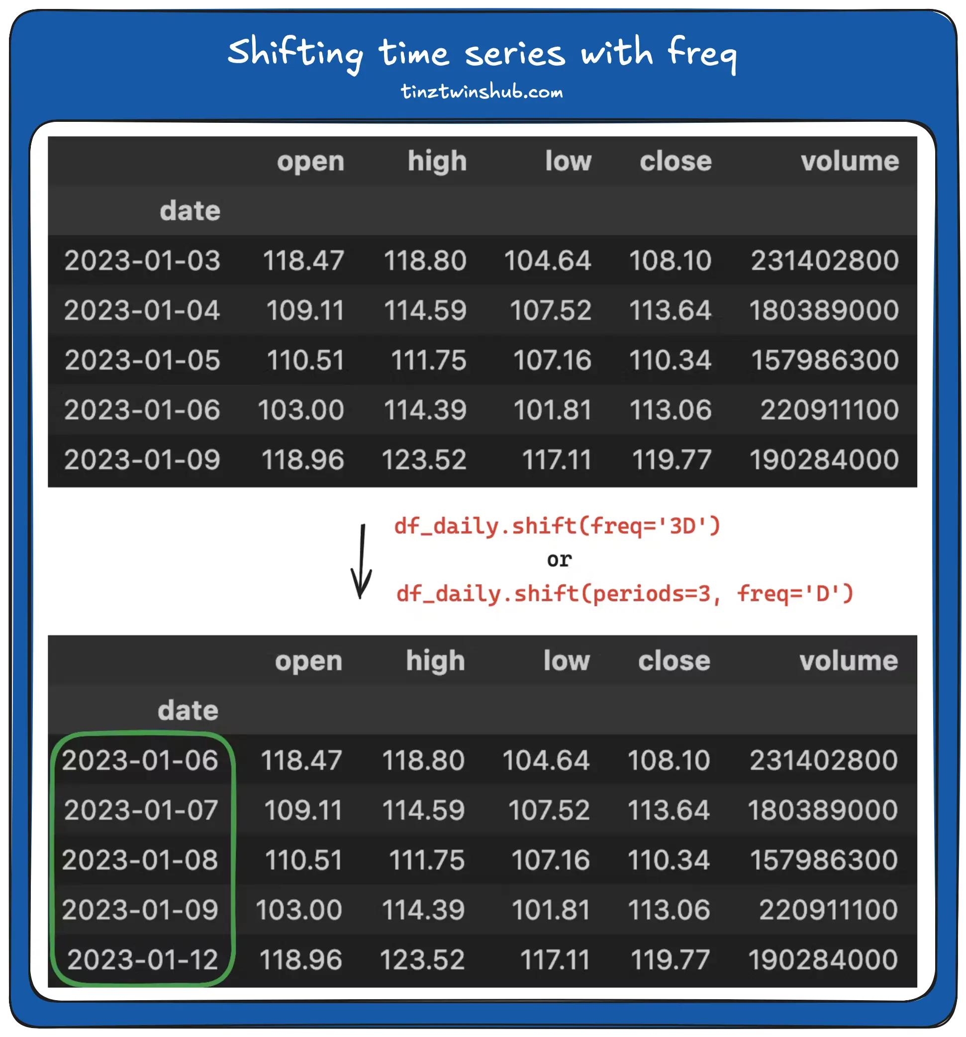
As a result, the entire time series data has been moved forward by three days. Additionally, there are no NaN values because we only shifted the index.

Difference between the closing prices of two consecutive days

Using the skills we’ve learned, we can now calculate the change in closing prices from one day to the next with the shift() function. Take a look at the code below.

df_daily['difference'] = df_daily['close'] - df_daily.shift(1)['close']

df_daily.head()

Output:

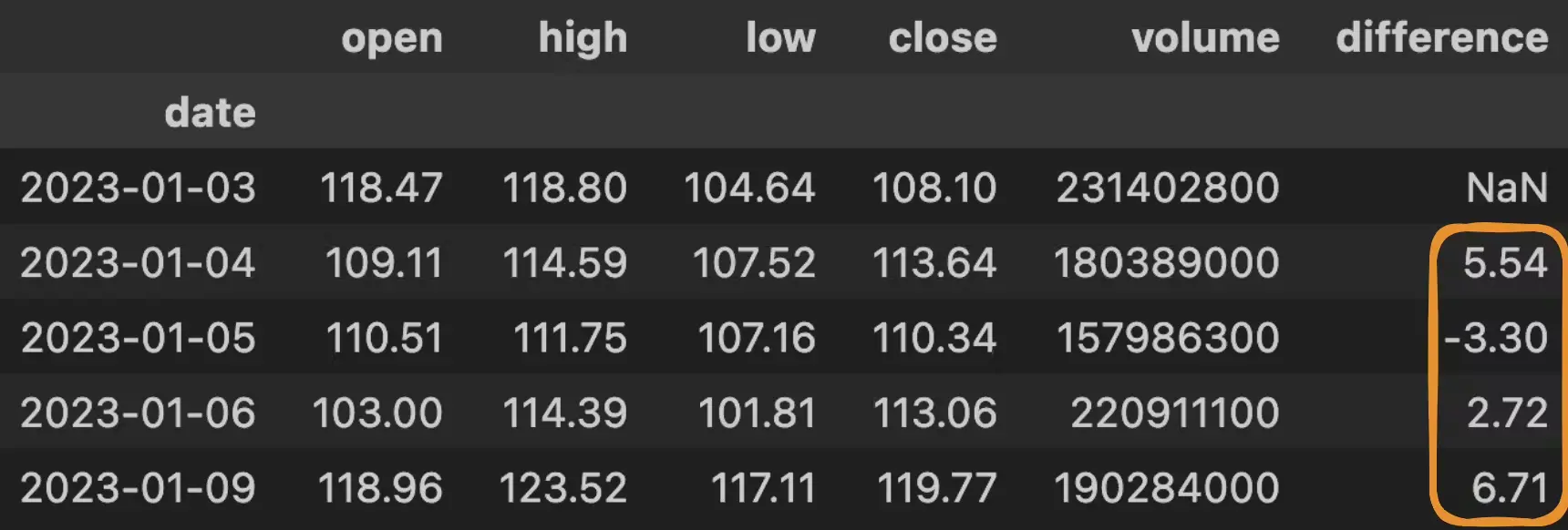
In the output dataframe, we can see the price change in the difference column, highlighted in orange. The first value in this column is NaN because there is no previous row to compare it with.

That’s it. Now, you can master time shifting in Pandas.

Conclusion

In this guide, we looked at how to use Pandas to work with stock market data, using Tesla as an example. We started by setting up our environment with OpenBB as our data source. We showed how to use the shift function in Pandas to move time series data forward or backward in time and to calculate the difference between data points.

Pandas make it easy to work with time series data in Python. It gives you the tools you need for financial market analysis. With these skills, you can do more with Python in finance and other areas.

---

💡 Do you enjoy our content and want to read super-detailed articles about data science topics? If so, be sure to check out our premium offer!

Premium Articles

---

Thanks so much for reading. Have a great day!